Code
library(anyflights)
library(dplyr)
The data used throughout this project deals with on-time performance of domestic flights within the United States. In the recent years, the air traffic has increased significantly and huge amounts of flight data is being generated each day. Hence, the data is filtered based on the following criteria:
The airports of interest are those serving the New York City (NYC) region (i.e. LGA, JFK, and EWR).
Both in-bound and out-bound domestic flights.
the data is restricted to the most recent year (i.e. 2023).
The data is obtained using the anyflights package from CRAN. This package queries the data released annually by the Federal Aviation Administration (FAA). The data for a particular year is released in the first quarter of the following year. The FAA database is updated every year and consequently the data can be queried from any historical data up to the most recent year. The data is obtained as five different data frames as follows:
flights: it provides all the daily flight on-time performance data. It includes the origin airport, scheduled departure time, destination airport, scheduled arrival time, carrier, tail number of the aircraft, arrival delay, and departure delay. It has 863228 rows and 19 columns.
weather: it provides hourly weather parameters for origin airport. These parameters include visibility, wind speed, pressure, precipitation, and humidity. It has 976340 rows and 15 columns.
planes: it provides the production information of an aircraft. It includes the tail number of the aircraft, year of manufacture, manufacturer, and the type of engine. It has 4848 rows and 10 columns.
airports: it provides the metadata for the airport. The metadata includes the FAA code, its name, time zone, latitude, longitude, and altitude. It has 1251 rows and 8 columns.
airlines: it provides the metadata for the airlines which is the IATA code of the carrier and its name. It has 14 rows and 2 columns.
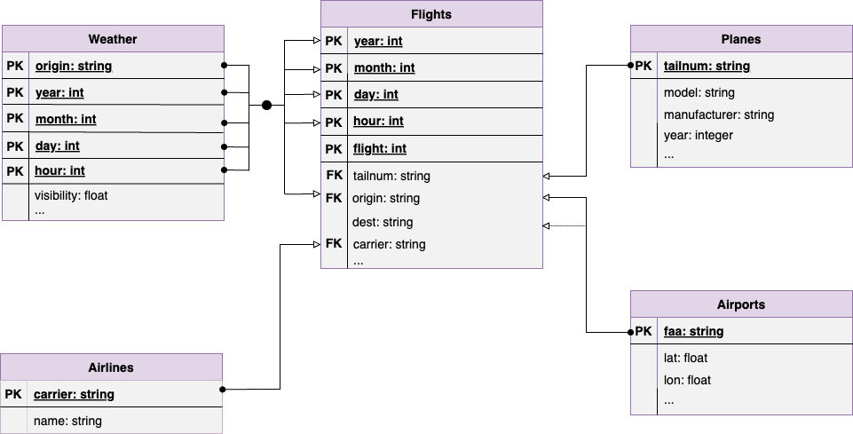
All the data frames are related to each other. Hence, the data has a relational structure. Every row in each of the data frames can be identified by a primary key (PK) and the flights data frame can related to each of the other four data frames with the help of foreign keys (FK). Figure 1 shows the relational schema of the data. For example, every entry in the flights data frame can be uniquely identified by (year, month, day, hour, and flight) and it can be joined with the weather data frame based on (origin, year, month, day, and hour)
The data used is not readily available online as CSV files. Hence, the data needs to be collected, filtered, consolidated, and saved for future use.
The next section describes the data preparation process.
The data collection includes two key steps:
Collection of data for out-bound flights from airports that serve NYC region.
Collection of data for in-bound flights from airports that serve NYC region.
To use the anyflights package it first needs to be installed using install.packages("anyflights") .
library(anyflights)
library(dplyr)The anyflights package has a anyflights() function which queries the FAA database. It fetches all the five aforementioned data frames and therefore it can take a lot of time to obtain the data contingent upon the network connectivity. In order to avoid chances of an API timeout, the default value of 60 seconds is updated with a high value of 1500 seconds stored in the API_REQ_TIMEOUT. All the previously stated constraints are stored in the STATIONS and YEAR constants. save_data() is a utility function to save the collected data into the required directory location.
# constants
API_REQ_TIMEOUT = 1500
STATIONS = c("LGA", "JFK", "EWR")
YEAR = 2023
DATA_DIR = "data"

# Utility function
save_data <- function(data, flight_type){

  tables <- c("flights", "planes", "airlines", "airports", "weather")
  csv_path <- ""

  for(table_name in tables){

    if(!any(table_name %in% c("airlines", "airports"))){

      csv_path = file.path(DATA_DIR, "raw", flight_type,
                           paste(table_name, "csv",
                                 sep = "."))
    }else{
      csv_path = file.path(DATA_DIR, "raw",
                           paste(table_name, "csv",
                                 sep = "."))
    }

    if(!file.exists(csv_path)){

      write.csv(x = data[table_name],
              file = csv_path)

      cat("Saved", paste(table_name, "csv",
                         sep = "."), "at",
          csv_path, "\n")

    }

  }

}For this use-case, an outbound flight is one that departs from one of airports that serve the NYC region and arrives at any other airport within the United States. Therefore, the departure airports denoted by the station argument is given the NYC airports and the year as 2023.
options(timeout = API_REQ_TIMEOUT)

nycflights23outbound <- anyflights::anyflights(station = STATIONS,
                                               year = YEAR)

save_data(data = nycflights23outbound,
flight_type = "outbound")For this use-case, an inbound flight is one that departs from any other airport within the United States (except the airports that serve the NYC region) and arrives at one of airports that serve the NYC region.
The departure airports are computed based on the distinct destination airports in flights data frame of nycflights23outbound . It happens to be that there are some airports for which the data cannot be fetched. Hence, the destination airports are filtered based on whether their FAA code appears in the faa column of airports data frame.
All the outbound flights are obtained for the computed list of airports. However, the flights data frame of nycflights23inbound consists of flights that depart and arrive at any airport within the United States. Therefore, all flights that do not arrive in the airports that serve NYC are filtered out based on the dest column of flights data frame.
all_airports <- nycflights23outbound$airports$faa

dest_airports <- nycflights23outbound$flights |>
                     filter(dest %in% all_airports & !dest %in% STATIONS) |>
                        select("dest") |>
                           unique()

dest_airports <- dest_airports$dest

nycflights23inbound <- anyflights::anyflights(station = dest_airports,
                                               year = YEAR)

nycflights23inbound$flights <- nycflights23inbound$flights |>
                                   filter(dest %in% STATIONS)

save_data(data = nycflights23inbound,
flight_type = "inbound")In the previous section, the data is collected into two different list: nycflights23inbound and nycflights23outbound . Each of these lists contain five data frames: flights, weather, planes, airports, and airlines. The airports and airlines data frames remain the same for inbound and outbound flights. The data for the flights, weather, and planes must be combined respectively.
All the rows in the inbound and outbound flights data frames are combined into a single data frame using rbind() powered by the dplyr package. The combined flights data is sorted based on the primary key of the flights table.
nycflights23 <- rbind(nycflights23inbound$flights,
                      nycflights23outbound$flights)

nycflights23 <- nycflights23 |>
                  arrange(year, month, day, hour, flight)

write.csv(x = nycflights23,
file = "data/raw/flights.csv")The weather data frame consists of the hourly weather parameters of the airport. The inbound and outbound weather data frames contain data for different set of airports. Therefore, both of them need to be joined in a similar way as that of flights data.
weather <- rbind(nycflights23inbound$weather,
                 nycflights23outbound$weather)

weather <- weather |>
             arrange(origin, year, month, day, hour)

write.csv(x = weather,
file = "data/raw/weather.csv")The planes data frame stored the production details for each aircraft based on its tailnum. Generally, the plane that operates the inbound flight also operates the outbound flight. However, since the NYC airports are hubs for a majority of US carriers, there is a possibility that an aircraft is changed for the onward flight.
Therefore, all the planes operating the inbound flights is considered and all planes for outbound flights that are not in set of planes that operated in the inbound flights are considered. At the end, the data is consolidate to get production details of all the aircraft operating on the routes in the flights data frame.
tailnum <- unique(nycflights23$tailnum)

planes_inbound <-
  planes_inbound |>
    filter(planes_inbound$planes.tailnum %in% tailnum)

planes_outbound <-
   planes_outbound |>
     filter(!planes_outbound$planes.tailnum %in% planes_inbound$planes.tailnum)

planes <- rbind(planes_inbound, planes_outbound)

write.csv(x = planes,
          file = "data/raw/planes.csv")
Finally, all the data is stored in /data directory under the /raw sub-directory since no data cleaning has been performed on it yet. The /raw sub-directory contains the .csv files for consolidated data and has two further sub-directories /inbound and /outbound with the respective .csv files.
library(tidyverse)── Attaching core tidyverse packages ──────────────────────── tidyverse 2.0.0 ──
✔ dplyr 1.1.4 ✔ readr 2.1.5
✔ forcats 1.0.0 ✔ stringr 1.5.1
✔ ggplot2 3.5.1 ✔ tibble 3.2.1
✔ lubridate 1.9.3 ✔ tidyr 1.3.1
✔ purrr 1.0.2
── Conflicts ────────────────────────────────────────── tidyverse_conflicts() ──
✖ dplyr::filter() masks stats::filter()
✖ dplyr::lag() masks stats::lag()
ℹ Use the conflicted package (<http://conflicted.r-lib.org/>) to force all conflicts to become errorslibrary(DataExplorer)
library(ggplot2)
library(dplyr)
library(purrr)airlines_data <- read.csv("data/raw/airlines.csv") |>
subset(select = -c(X))
# head(airlines_data)
airports_data <- read.csv("data/raw/airports.csv") |>
subset(select = -c(X))
# head(airports_data)
flights_data <- read.csv("data/raw/flights.csv") |>
subset(select = -c(X))
# head(flights_data)
planes_data <- read.csv("data/raw/planes.csv") |>
subset(select = -c(X, X.1))
# head(planes_data)
weather_data <- read.csv("data/raw/weather.csv") |>
subset(select = -c(X))
# head(weather_data)# missing values in airline data
airlines_data |> plot_missing(title = "Missing Values in Airlines Data")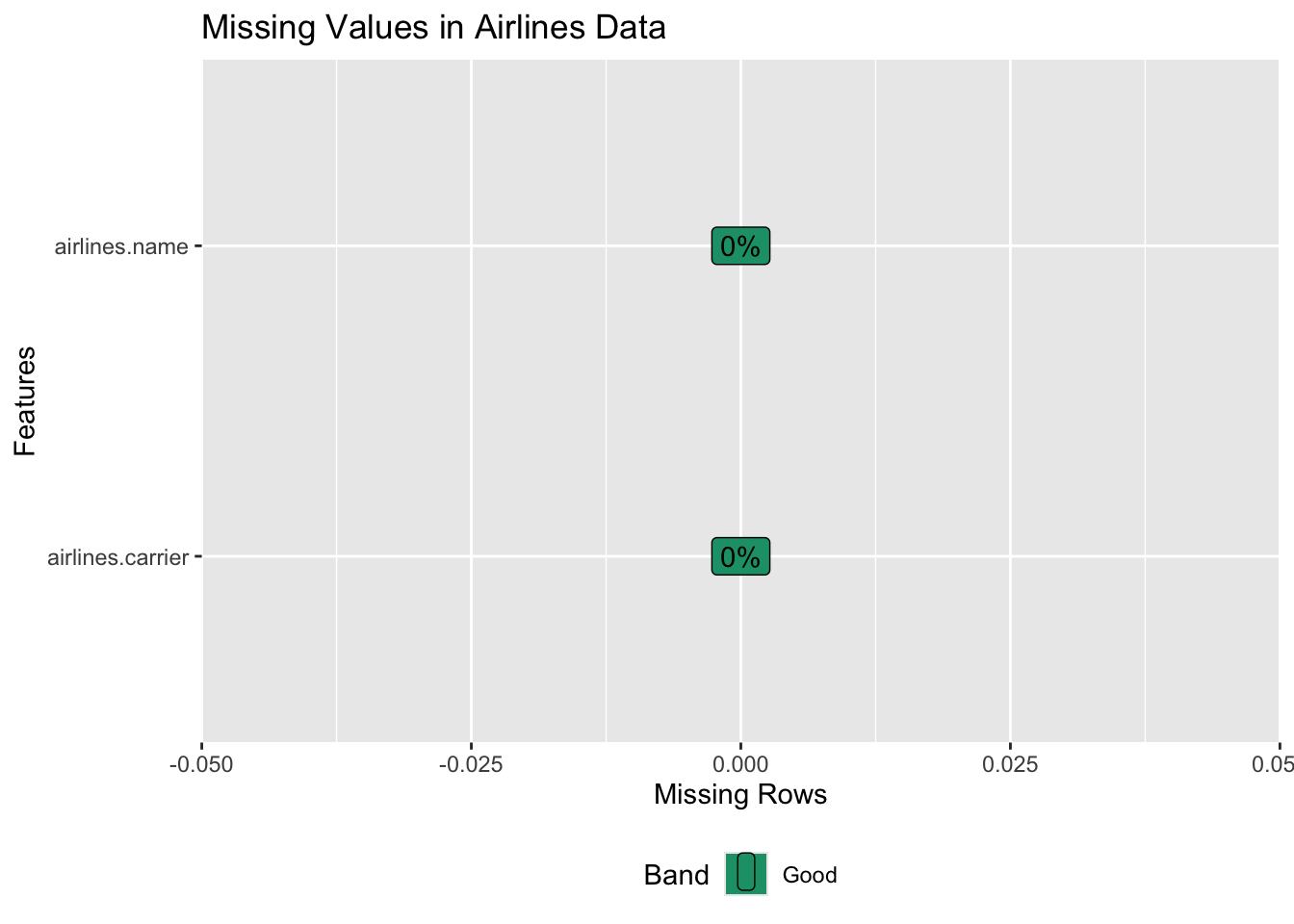
# missing values in airports data
airports_data |> plot_missing(title = "Missing Values in Airports Data")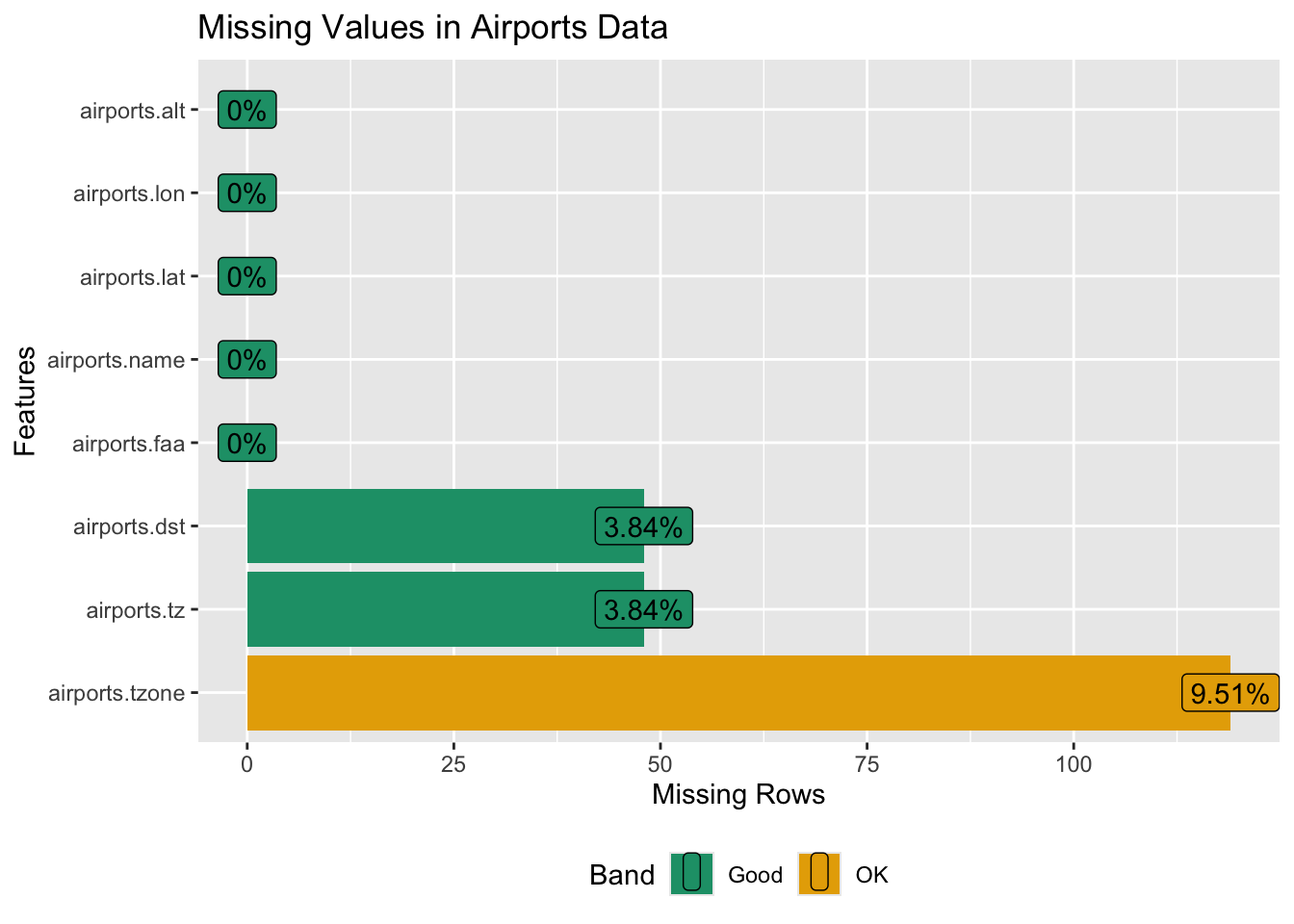
# missing values in flights data
flights_data |> plot_missing(title = "Missing Values in Flights Data")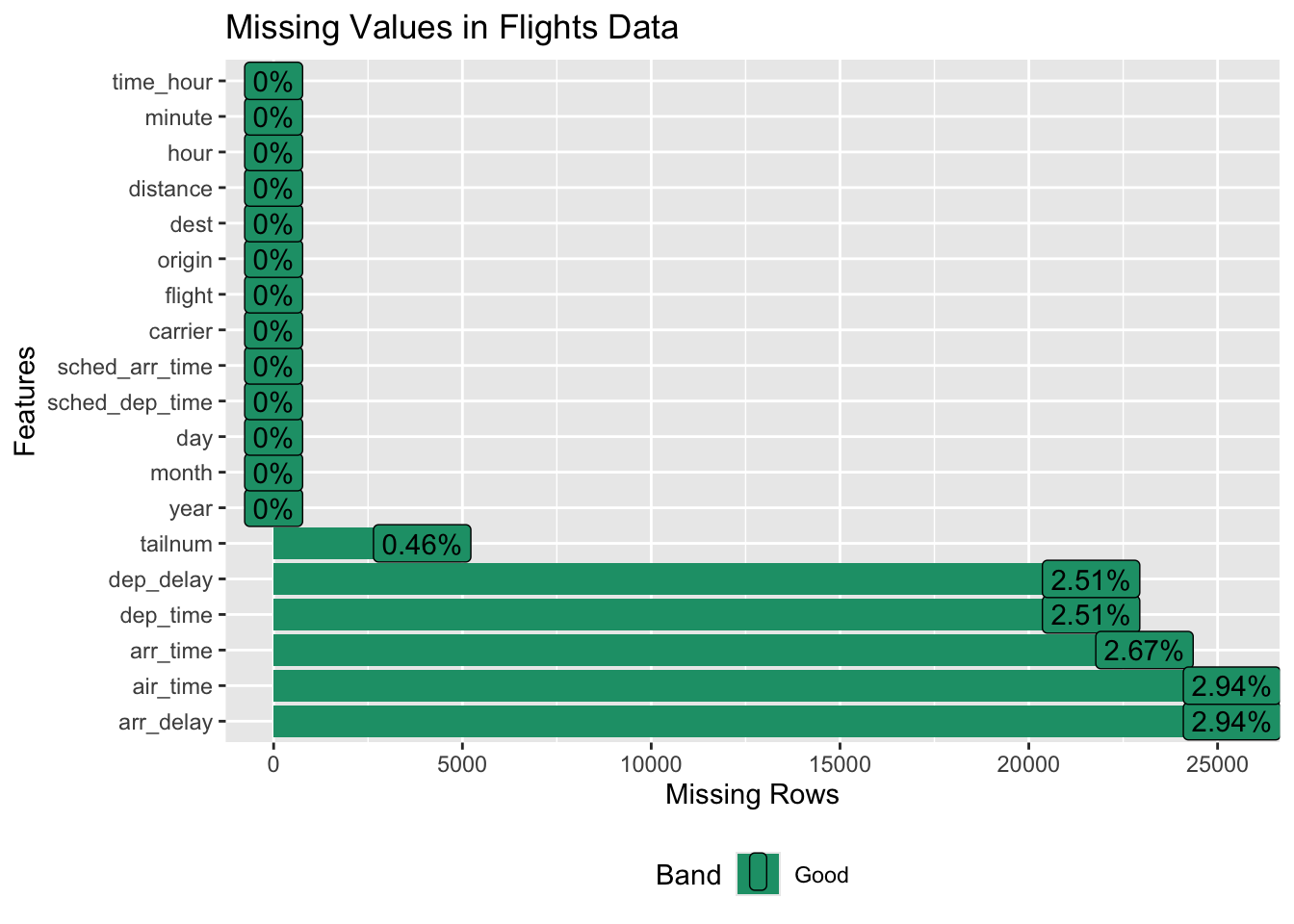
# missing values in planes data
planes_data |> plot_missing(title = "Missing Values in Planes Data")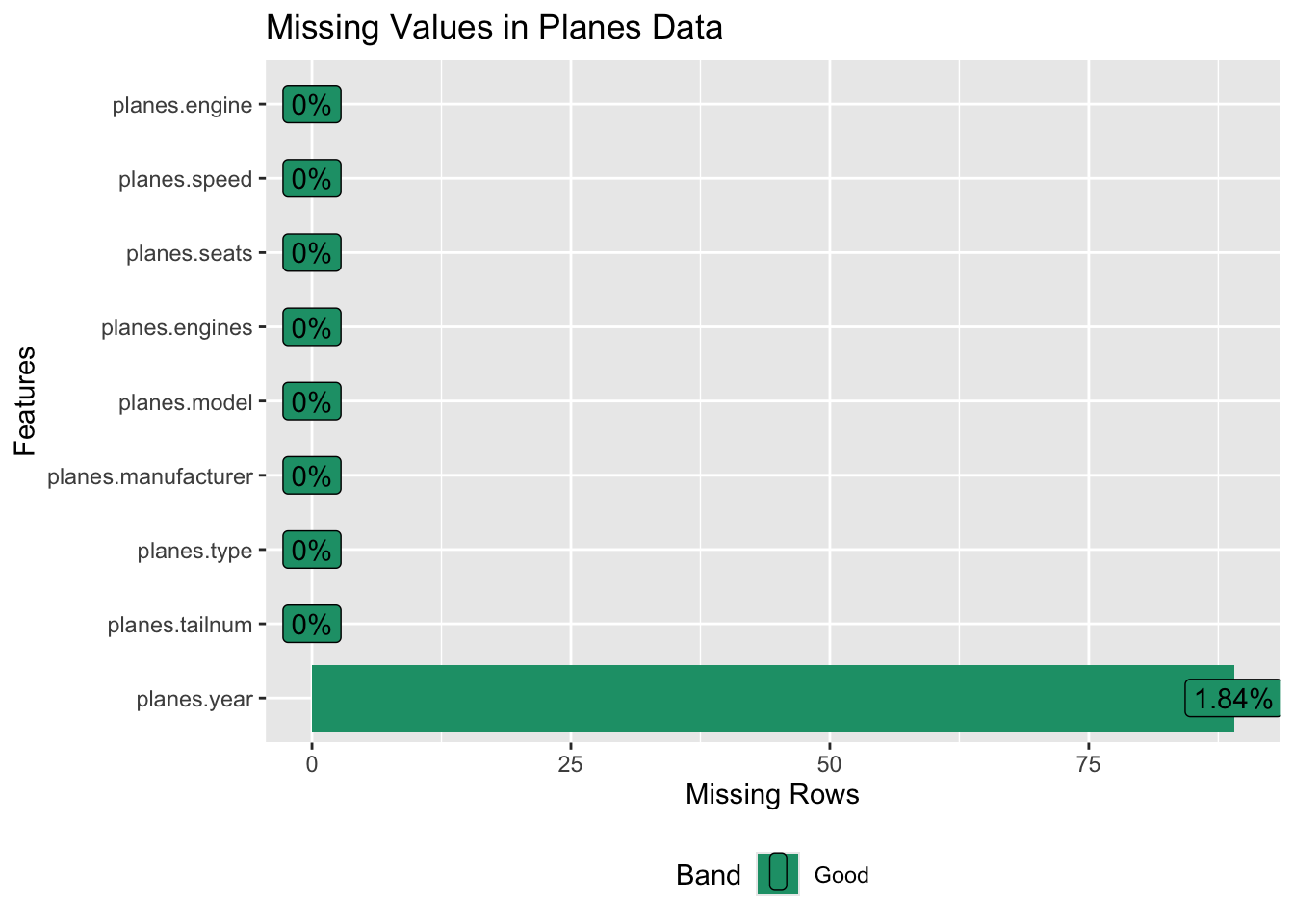
# missing values in weather data
weather_data |> plot_missing(title = "Missing Values in Weather Data")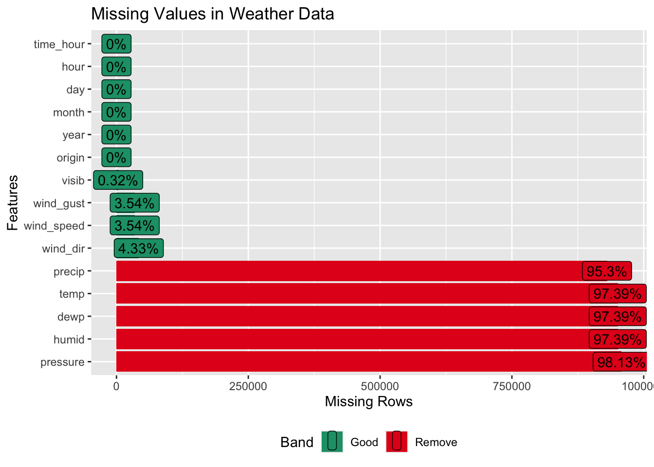
The airlines_data stores the airline code and name. Hence, it does not have any null values
The airports_data has 9.51% missing values in airports.tzone column. However, it can be derived from the airports.tz column
Flights_data has null values for actual time of departure and arrival. However, there are no null values in the scheduled time of departure and arrival.
In the planes_data, the year column has null values which do not have any significance behind them.
The weather_data however has several missing values. In fact, more than 95% of the values are missing in 5 of the columns - precip, temp, deep, humid, pressure. Thus, these features may be dropped.
datasets <- list(
  airlines = airlines_data,
  airports = airports_data,
  flights = flights_data,
  planes = planes_data,
  weather = weather_data
)

# Calculate missing values for each dataset
missing_summary <- map_dfr(datasets, ~ {
  data.frame(
    Dataset = deparse(substitute(.x)),
    Total_Values = prod(dim(.x)),
    Missing_Values = sum(is.na(.x)),
    Proportion_Missing = sum(is.na(.x)) / prod(dim(.x))
  )
}, .id = "Dataset")

# Plot comparison of missing values
ggplot(missing_summary, aes(x = Dataset, y = Proportion_Missing, fill = Dataset)) +
  geom_col(show.legend = FALSE) +
  geom_text(aes(label = scales::percent(Proportion_Missing, accuracy = 0.1)),
            vjust = -0.5,
            size = 4) +
  scale_y_continuous(labels = scales::percent) +
  labs(
    title = "Proportion of Missing Values Across Datasets",
    x = "Dataset",
    y = "Proportion of Missing Values"
  ) +
  theme_minimal()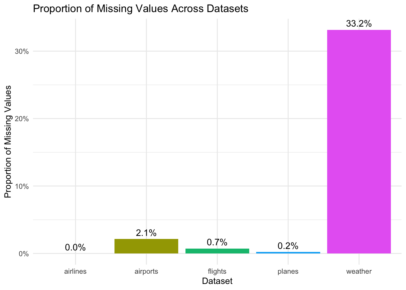
Weather_data has a high percentage of missing values (33.2%) while the rest of the data has barely any missing values.
However, most of the missing values for weather_data are concentrated among 5 features.
Hence, after we remove these 5, the proportion of missing values for weather will come down drastically.
library(redav)
Attaching package: 'redav'The following object is masked from 'package:DataExplorer':
plot_missingmv_cols <- c("dep_delay", "arr_delay", "arr_time", "dep_time",
"air_time", "tailnum")
plot_missing(flights_data[mv_cols], percent = TRUE)Scale for y is already present.
Adding another scale for y, which will replace the existing scale.Scale for y is already present.
Adding another scale for y, which will replace the existing scale.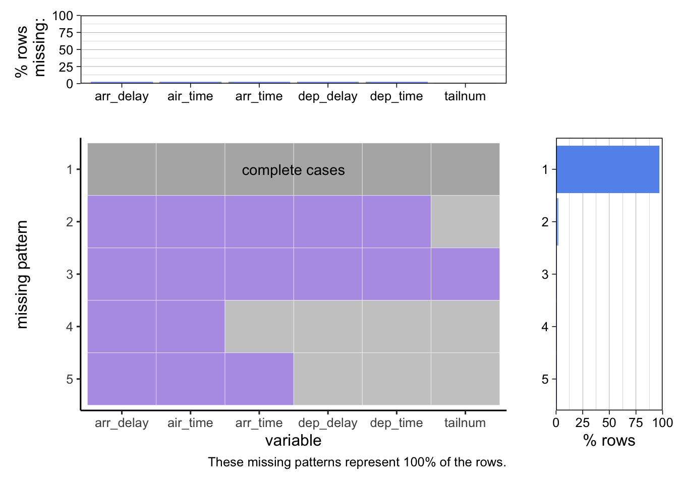
There three noticeable patterns in missing values in the flights data frame:
The first case is of a cancellation before aircraft allocation when all the six columns are missing.
The second case is of a cancellation after aircraft allocation when all the columns except tailnum are missing.
The third case is of a diversion when the arr_delay, arr_time, and air_time are missing. This implies that the aircraft was scheduled to arrive but did not arrive.
However, in the fourth case, it is possible (but not certain) that the plane took off and faced a technical issue and landed back to the origin or one of NYC airports.